We all know and appreciate the fact that fuel injection/delivery strategies on petrol engines are based on the volume of atmospheric air that enters an engine. We also appreciate the fact that in order for an ECU to maintain a stoichiometric fuel mixture, that ECU has to be able to compensate for variations in intake air temperatures, and therefore intake air densities, as well as for variations in the speed at which intake air enters the engine. While there are several ways of accomplishing all of these, this article will focus on the basic science of measuring mass airflow rates, but with a particular emphasis on how MAF sensors measure mass airflow rates, starting with explaining-
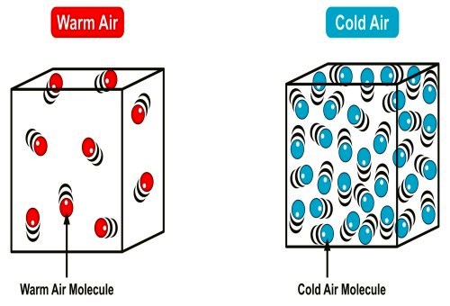
From an engine management systems’ perspective, the problem with atmospheric air is that the density of air in any given volume varies hugely according to temperature, and elevation above sea level.
The image above describes the point perfectly; the hotter atmospheric air becomes, the less dense it becomes. However, there is an additional complication, which is the fact that although atmospheric pressure declines smoothly by 1.2 KPa for every 100-metre increase in elevation above sea level, this applies only to relatively low altitudes on the one hand, and does not include variations caused by temperature inversions or humidity levels, on the other.
We need not delve into the complexities of what exactly causes variations in atmospheric pressure here, but suffice to say that the variable nature of atmospheric pressures at different altitudes present engine designers with rather a thorny problem. For instance, engine and fuel management systems that produce “X” number of kilowatts from an engine at sea level, also have to produce “X” number of kilowatts from the same engine at an elevation of say, 1 500 metres above sea level, where the atmosphere is appreciably less dense than it is at sea level.
Essentially, the problem is this; since the atmospheric pressure, and therefore, the amount of air that is available to an engine at any given altitude cannot be changed to suit a particular engine’s requirements, how does a fuel management system on a petrol engine maintain a stoichiometric air/fuel mixture at all altitudes?
We know that at stoichiometric ratios on petrol engines, all the fuel is combusted using all of the available air, but since the amount of air varies greatly, the only factor that can be changed or adapted relative to the amount of available air is the amount of fuel that is delivered to the cylinders. Making such an arrangement work however, requires precise measurement of the amount of air that enters the engine, and although the mass of petrol is known, the mass of the intake air varies, so engine designers had to find a way to correlate the volume of the intake air to its mass, which are two different things.
Nonetheless, since the mass of petrol is known, engine designers have developed three distinctly different methods of measuring and/or calculating the mass of the air that enters an engine at any given moment, these being the-
Alpha-n method
This method uses primary input data from the throttle position sensor. In practice, the fuel management system uses pre-programmed look-up tables to derive the mass value for the intake air based on the effective throttle opening.
While this method works reasonably well, the look-up tables cannot compensate for pulsation errors, nor can it compensate for variations in temperature and humidity, both of which have a direct bearing on the density of the intake air.
Speed density method
These systems use primary input data from a MAP (Manifold Absolute Pressure) sensor. In terms of operating principles, the speed density method uses look-up tables to derive a mass value for the intake air based on the absolute pressure within the intake manifold at any given moment.
However, the biggest disadvantage of the speed density method is that it cannot compensate for variations in the engines’ volumetric efficiency. For instance, if a restriction in the exhaust system exists that affects the efficient extraction of exhaust gases, the pressure within the intake manifold will necessarily increase toward atmospheric pressure. As a practical matter, the ECU will interpret this situation as the volume of air entering the engine being more massive than it really is which will result in a reduction of the injector pulse widths to produce an inappropriate negative fuel trim value.
Mass airflow measurement method
This method uses input data from the MAF sensor to derive a mass value for the intake air. Unlike other methods though, MAF sensors use look-up tables that are based on the rate of airflow through the induction system, as opposed to the possible (and often, assumed) volume of air that enters the engine.
While all three airflow-measurement methods have advantages and disadvantages, many modern engine and fuel management systems use at least some aspects of all three systems, regardless of the primary system in use. Thus, from a diagnostic perspective, it is important to determine which primary system is in use, since each method of determining the mass of intake air affects fuel injection systems differently.
This is especially true of drive-by-wire throttle control systems that use the Alpha-n or speed density methods. In these cases, the time delay in throttle actuations can produce large, but momentary swings in fuel trim values that can sometimes be easy to misinterpret as slow response times by oxygen or air/fuel ratio sensors.
Similarly, while systems that use MAF sensors typically have excellent throttle response times and do not suffer from the effects of altitude variations, nor influences caused by humidity or pulsation errors, these systems can sometimes still suffer from a significant time delay factor. Moreover, since the accuracy of MAF sensors are severely affected by turbulence in the inlet ducting, such as might occur during hard accelerations, fuel management systems typically do not use primary input data from MAF sensors during fast (and large) changes in the throttle plate position.
Nonetheless, despite the shortcomings of MAF sensors, these systems still offer many distinct and tangible benefits and advantages over other types of systems, so let us look at these systems in more detail, starting with-
Early iterations of MAF sensors were fairly simple devices that used the airflow through them to open a sort of trap door that was connected to a simple potentiometer. Since the potentiometer was calibrated to register closed and open positions, any position between these two positions was directly proportional to the volume of air that flowed through the sensor.
These early sensors took no account of the temperature or humidity of intake air, but they had the advantage that they did not suffer from air density issues. In practice, since the force of the air moving through the sensor acted on the trap door, which caused the potentiometer to pass a varying signal voltage to the ECU, it was a fairly simple matter for the ECU to calculate the volume of air entering the engine, based on the signal voltage being passed back to the ECU. Thus, assuming that the trapdoor responded consistently, the ECU was able to make consistently appropriate adaptations to the injector pulse width since the volume, and by inference, the mass of the air entering the engine was known to within a few percent.
However, as emissions regulations became ever more stringent, simple trap door MAF sensors became unsuited to the exacting requirements of multiple injection and sparking systems, neither of which worked well in the absence of a way to make almost real-time adjustments to the air/fuel mixture. Essentially, what was needed was a way to measure airflow through the intake system more accurately by taking into account the effects of ambient temperature and humidity on the density of the intake air, while eliminating the effects of pulsating pressure waves within the intake system and elevation above sea level, at the same time.
All of the above is a very tall order, but engineers have found a way to use convection as a means to measure airflow rates, which brings us to-
Convection is most easily described as a mechanism of heat transfer through the movement of fluids or gases, the gas in the case of MAF sensors being atmospheric air. In their simplest form, heated element MAF sensors are fitted with heated elements in the form of a wire or metal film that is placed directly in the path of the air that moves through the sensor. As the air moves through the sensor, the moving air has a cooling effect on the heated element or film in exactly the same way that we experience a drop in temperature when the wind blows.
This is known as the “wind chill” factor, but as it applies to MAF sensors, the number of air molecules in any given cubic volume has a direct bearing on the degree of cooling of the heated element that takes place. Put in another way, this means that if the air is cold and dense, more air molecules come into contact with the heated element than would have been the case had the air been warm and less dense. As a practical matter then, the more air molecules that come into contact with the heated element, the greater the cooling effect, which is rather fortunate since as far as the ECU is concerned, this largely eliminates altitude, humidity, and temperature variations in the intake air. Here is why-
In terms of operating principles, the element in the MAF sensor is supplied with a constant current that keeps the element heated to a constant temperature, which is typically between 425 Centigrade, and 230 degrees Centigrade and to eliminate time delay issues, MAF sensor elements are constructed from platinum wire that is about 0.7 mm in diameter to ensure rapid heat transfer to the airflow. In terms of control, the heated element’s resistance is monitored continuously; as heat is removed from the element its resistance decreases, but when the air flow diminishes, the element’ resistance increases.
In practice, a bridging circuit supplies the element with a current of between 500 milliamps and 1500 milliamps, which is also monitored on a continuous basis. Thus, when the airflow through the sensor increases, progressively more heat is removed from the element, which changes the element’s resistance, which in turn, causes the ECU to supply more current to the element in order to restore or maintain the element’s target temperature. As a practical matter, this means that the elements’ temperature and resistance are functions of the volume of air that flows through the sensor. Therefore, based on the volume of air flowing through the MAF sensor, as well as the relationship between amount of heat lost through convection and the current required to maintain the elements’ temperature, the ECU is able to infer the mass of the intake air, and from there, complex algorithmic calculations are used to determine an appropriate injector pulse width.
However, since engines with different displacements require differing volumes of air to work efficiently, engine designers simply match the diameter of the MAF sensor to a particular engine displacement, based on the calculated volumetric efficiency of the engine. The practical advantage of this is the fact that engine designers do not have to develop and calibrate MAF sensor elements and resistors for each new engine, since the airflow remains the same per unit of time, regardless of engine displacement. Thus, by simply making the diameter of the MAF sensor bigger or smaller to suit a new engine design, the same elements and resistors can be used across all applications with consistently accurate results.
While simple heated element MAF sensors work well, the latest iterations of MAF sensors use an additional temperature correction circuit. This circuit incorporates a dedicated correction resistor that is made from platinum foil or film that has a typical resistance of 500 ?. The primary function of this resistor is to compensate for variations in the MAF sensor’s bridging circuit that occur during mass-production, so in practice, each individual temperature compensating resistor is precision-trimmed with lasers to ensure proper calibration of the bridging circuit. A second laser-trimmed resistor is used both to compensate for variations in the element’s heating circuit, and to calibrate the sensors’ temperature monitoring circuit.
Additionally, many MAF sensors incorporate a barometric pressure sensor to serve as a back-up device that can supply the engine with basic airflow data when the MAF sensor fails.
As we know, many things can go wrong with MAF sensors, but finding the root cause of some MAF sensor failures is not always easy. In fact, since even microscopic damage to a heated element can cause a MAF sensor to report inaccurate airflows, it is sometimes easier and quicker simply to perform a volumetric efficiency test on a suspect MAF sensor, than it is to hunt down issues that may or may not be the root cause of for instance, unacceptably high or low fuel trim values.
MAF sensor volumetric tests are based on the assumption that an engine of a given displacement will move an amount of air that is equal to the engines’ displacement during two full engine revolutions. However, factors like the ambient air temperature and pressure, engine speed, the efficiency of the air filter, and restrictions in the exhaust system (among many others) all detract from the volume of air an engine can “pump” during two revolutions.
Nonetheless, since all high-end diagnostic computers that incorporate oscilloscopes have the ability to create a trace of an engines’ theoretical volumetric efficiency, it is a simple matter to compare that trace with a simultaneous trace obtained from the MAF sensor. If the MAF sensor is fully functional, its trace will match the engine’s volumetric trace very closely. This is especially true of snap-throttle events that produce large variations in the MAF sensors’ signal voltage, but note that as mentioned elsewhere, drive-by-wire throttle control systems may exhibit a significant time delay between the two traces.
Note that if readings of a fully functional MAF sensors’ output voltage is taken at multiple points from idle to wide-open throttle, fuel trim values should never exceed acceptable levels. Note also that on a fully functional MAF sensor, the change in the signal voltage from minimum to maximum should always be greater than 2.5 volts, which is 50% of the sensors’ reference voltage.
Defective (or sometimes, rebuilt and some aftermarket) MAF sensors on the other hand, will typically display signal voltage changes that are less than 2.5 volts, which will almost always be accompanied by unacceptably high or low fuel trim values, since the ECU will attempt to compensate for incorrectly reported airflows through the MAF sensor.
Once you understand how modern MAF sensors work, it becomes a great deal easier to diagnose issues that either affect their operation, or to accurately interpret symptoms that are caused by defective MAF sensors. Either way, one of the most effective ways to diagnose these issues is to collect as many known good MAF oscilloscope traces as you can, which you can do simply by connecting an oscilloscope scope to vehicles you are servicing or otherwise working on, and saving the results. If you do this consistently and on as many different vehicles as you can, you will soon build up a comprehensive MAF sensor waveform library that will make diagnosing future MAF issues a whole lot easier, quicker, and more profitable.